
Q. What do you mean by expected frequencies in (a) chi-square test for testing independence of attributes, and (b) chi-square test for testing goodness-of-fit? Also explain the procedure you follow in calculating the expected values in each of the above situations.
Expected Frequencies in
Chi-Square Tests
Chi-square tests are
statistical tests used to examine the association between categorical
variables. The expected frequencies represent the frequency of occurrences that
we would expect in each category of a contingency table if there were no
association between the variables. In both the Chi-Square Test for
Independence and the Chi-Square Test for Goodness-of-Fit, expected
frequencies are calculated based on the assumption that there is no significant
effect or relationship between the variables being studied. The procedure for
calculating expected frequencies differs slightly between the two tests, and
understanding the methodology is crucial for performing these tests correctly.

(a) Chi-Square Test for
Testing Independence of Attributes
The Chi-Square Test
for Independence is used to determine whether two categorical variables are
independent or related. For example, you might use this test to determine
whether gender (male/female) and preference for a particular type of movie
(action/comedy/drama) are independent or associated. The test is performed by
comparing the observed frequencies in a contingency table with the expected
frequencies under the assumption that the variables are independent.
Procedure for Calculating
Expected Frequencies in the Chi-Square Test for Independence
1. Create
a Contingency Table:
The first step is to organize the observed data into a contingency table, where
rows represent the categories of one variable (e.g., gender) and columns
represent the categories of the second variable (e.g., movie preference). Each
cell in the table contains the observed frequency of occurrences in that
particular category combination.
2. Calculate
the Row and Column Totals:
Compute the sum of observations in each row and column of the table. These
totals are necessary to calculate the expected frequencies.
3. Calculate
the Grand Total:
The grand total is the sum of all the observed frequencies in the table. This
total represents the total number of observations across all categories.
4. Calculate
the Expected Frequencies:
The expected frequency for each cell in the contingency table is calculated
using the following formula:
Eij=(Row Total)i×(Column Total)jGrand TotalE_{ij}
= \frac{(Row\ Total)_{i} \times (Column\ Total)_{j}}{Grand\ Total}Eij=Grand Total(Row Total)i×(Column Total)j
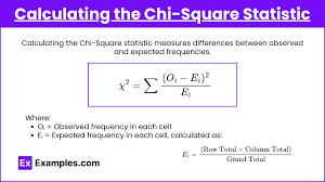
Where:
o EijE_{ij}Eij
is the expected frequency for the cell in the iii-th row and jjj-th column,
o (Row Total)i(Row\
Total)_{i}(Row Total)i is the total for the iii-th row,
o (Column Total)j(Column\
Total)_{j}(Column Total)j is the total for the jjj-th column,
o Grand TotalGrand\
TotalGrand Total is the total number of observations in the table.
The expected frequency
represents the number of observations we would expect in each cell if the two
variables were independent. For example, if you are testing the independence of
gender and movie preference, the expected frequency for a particular combination
of gender and movie type would be the product of the total number of males (row
total) and the total number of people who prefer action movies (column total),
divided by the total number of people in the study.
5. Repeat
the Calculation for All Cells:
The expected frequency must be calculated for each cell in the contingency
table. Once all expected frequencies are computed, they are compared with the
observed frequencies.
6. Chi-Square
Test Statistic Calculation:
After calculating the expected frequencies, the Chi-Square test statistic (χ2\chi^2χ2)
is calculated using the formula:
χ2=∑(Oij−Eij)2Eij\chi^2 =
\sum \frac{(O_{ij} - E_{ij})^2}{E_{ij}}χ2=∑Eij(Oij−Eij)2
Where:
o OijO_{ij}Oij
is the observed frequency for the iii-th row and jjj-th column,
o EijE_{ij}Eij
is the expected frequency for the iii-th row and jjj-th column,
o The
sum is taken over all cells in the table.
7. Degrees
of Freedom:
The degrees of freedom (df) for the Chi-Square test for independence are
calculated as:
df=(r−1)×(c−1)df = (r -
1) \times (c - 1)df=(r−1)×(c−1)
Where:
o rrr
is the number of rows in the table,
o ccc
is the number of columns in the table.
8. Hypothesis
Testing:
Finally, the Chi-Square test statistic is compared with the critical value from
the Chi-Square distribution table for the calculated degrees of freedom and
chosen significance level (alpha). If the test statistic exceeds the critical
value, we reject the null hypothesis, indicating that the two variables are not
independent.
Example of Chi-Square
Test for Independence
Suppose we are testing
whether there is an association between gender and preference for three types
of movies: action, comedy, and drama. We collect data on 300 individuals, and
we organize it into a contingency table:
|
Action |
Comedy |
Drama |
Row
Total |
|
|
Male |
60 |
30 |
10 |
100 |
|
Female |
50 |
80 |
70 |
200 |
|
Column
Total |
110 |
110 |
80 |
300 |
The expected frequency
for males who prefer action movies is:
E11=(100×110)300=36.67E_{11}
= \frac{(100 \times 110)}{300} = 36.67E11=300(100×110)=36.67
This calculation would be
repeated for each cell in the table.
(b) Chi-Square Test for
Goodness-of-Fit
The Chi-Square
Goodness-of-Fit Test is used to determine how well an observed distribution
fits an expected distribution. This test is commonly used to compare the
observed frequencies of categories in a sample to the expected frequencies
based on a known distribution. For example, you might use this test to
determine whether a die is fair by comparing the observed frequencies of the
numbers rolled to the expected frequencies under the assumption of a fair die
(i.e., each number has an equal chance of occurring).
Procedure for Calculating
Expected Frequencies in the Chi-Square Test for Goodness-of-Fit
1. State
the Null and Alternative Hypotheses:
The null hypothesis typically states that the observed frequencies match the
expected frequencies according to the hypothesized distribution. The
alternative hypothesis posits that there is a significant difference between
the observed and expected frequencies.
o Null
Hypothesis (H₀): The observed distribution follows the
expected distribution.
o Alternative
Hypothesis (H₁): The observed distribution does not
follow the expected distribution.
2. Determine
the Expected Frequencies:
To calculate the expected frequencies, we must first determine the total number
of observations. The expected frequency for each category is calculated by
multiplying the total number of observations by the proportion expected under
the hypothesized distribution. If we are testing whether a die is fair, the
expected frequency for each of the six faces of the die is:
Ei=Total Number of RollsNumber of CategoriesE_i
= \frac{Total\ Number\ of\ Rolls}{Number\ of\ Categories}Ei=Number of CategoriesTotal Number of Rolls
For example, if we roll a
die 120 times, the expected frequency for each face (if the die is fair) would
be:
Ei=1206=20E_i =
\frac{120}{6} = 20Ei=6120=20
This formula assumes that
each category (or face of the die) has an equal probability of occurring, which
is the case for a fair die.
3. Calculate
the Chi-Square Statistic:
The Chi-Square test statistic is calculated by comparing the observed
frequencies (OiO_iOi) to the expected frequencies (EiE_iEi) using the
formula:
χ2=∑(Oi−Ei)2Ei\chi^2 =
\sum \frac{(O_i - E_i)^2}{E_i}χ2=∑Ei(Oi−Ei)2
Where:
o OiO_iOi
is the observed frequency for the iii-th category,
o EiE_iEi
is the expected frequency for the iii-th category,
o The
sum is taken over all categories.
4. Degrees
of Freedom:
The degrees of freedom for the Chi-Square Goodness-of-Fit Test are calculated
as:
df=k−1df = k - 1df=k−1
Where:
o kkk
is the number of categories.
5. Hypothesis
Testing:
After calculating the test statistic, compare the value with the critical value
from the Chi-Square distribution table for the given degrees of freedom and
significance level. If the test statistic exceeds the critical value, the null
hypothesis is rejected, indicating that the observed distribution significantly
differs from the expected distribution.
Example of Chi-Square
Test for Goodness-of-Fit
Suppose we roll a fair
die 120 times, and the observed frequencies of the six faces are as follows:
|
Face |
Observed
Frequency (O) |
|
1 |
18 |
|
2 |
22 |
|
3 |
20 |
|
4 |
25 |
|
5 |
15 |
|
6 |
20 |
The expected frequency
for each face, assuming the die is fair, is:
Ei=1206=20E_i =
\frac{120}{6} = 20Ei=6120=20
The Chi-Square statistic
is calculated as:
χ2=(18−20)220+(22−20)220+(20−20)220+(25−20)220+(15−20)220+(20−20)220\chi^2
= \frac{(18-20)^2}{20} + \frac{(22-20)^2}{20} + \frac{(20-20)^2}{20} +
\frac{(25-20)^2}{20} + \frac{(15-20)^2}{20} + \frac{(20-20)^2}{20}χ2=20(18−20)2+20(22−20)2+20(20−20)2+20(25−20)2+20(15−20)2+20(20−20)2
χ2=(−2)220+2220+0220+5220+(−5)220+0220\chi^2 = \frac{(-2)^2}{20} +
\frac{2^2}{20} + \frac{0^2}{20} + \frac{5^2}{20} + \frac{(-5)^2}{20} +
\frac{0^2}{20}χ2=20(−2)2+2022+2002+2052+20(−5)2+2002 χ2=420+420+0+2520+2520+0=1.4+1.4+0+1.25+1.25+0=5.3\chi^2
= \frac{4}{20} + \frac{4}{20} + 0 + \frac{25}{20} + \frac{25}{20} + 0 = 1.4 +
1.4 + 0 + 1.25 + 1.25 + 0 = 5.3χ2=204+204+0+2025+2025+0=1.4+1.4+0+1.25+1.25+0=5.3
The degrees of freedom
are df=6−1=5df = 6 - 1 = 5df=6−1=5, and we compare the test statistic to the
critical value from the Chi-Square distribution table with 5 degrees of freedom
at a significance level of 0.05.
Conclusion
Both the Chi-Square
Test for Independence and the Chi-Square Goodness-of-Fit Test
involve calculating expected frequencies, but the methods for doing so depend
on the context of the test. In the Chi-Square Test for Independence, the
expected frequencies are calculated based on the assumption that the two
categorical variables are independent. In the Chi-Square Goodness-of-Fit Test,
the expected frequencies are based on the hypothesized distribution of the
categories. By calculating these expected frequencies and comparing them to the
observed frequencies, researchers can test hypotheses about the relationship
between categorical variables or the fit of observed data to a theoretical
distribution.


0 comments:
Note: Only a member of this blog may post a comment.